
Lambda Architecture in Action - From Sensors to Dashboards with Kafka, Iceberg, Nessie, StarRocks, Minio, Mage, and Docker
End-To-End implementation of IoT data pipeline using Lambda Architecture.


Hello again, fellow technology enthusiasts!
As data engineers, our mission is to design, build, and maintain robust data pipelines that efficiently meet business needs, among other responsibilities. But as data volumes grow and real-time demands increase, choosing the right architecture becomes challenging. Over the years, a few patterns have emerged as go-to solutions — most notably, the Lambda and Kappa architectures.
In this post, I’ll walk you through an end-to-end implementation of the Lambda architecture in a hypothetical (but practical!) business scenario. We’ll explore its core components, trade-offs, and how it balances batch and real-time processing. Stay tuned — in a follow-up post, I’ll tackle the same use case with Kappa architecture to compare the two approaches.
Ready to dive in? Let’s get started!
Introduction to Lambda Architecture
Lambda architecture is a data processing framework that handles massive datasets by combining batch processing (for accuracy and completeness) with real-time stream processing (for low-latency insights). Introduced by Nathan Marz and James Warren, this architecture addresses the limitations of traditional batch-only systems by splitting data processing into three layers (1 and 2 are the main differentiators from Kappa Architecture):
Batch Layer — Processes historical data in large batches, ensuring accuracy and completeness. (Demo tech: Apache Iceberg on MinIO with Nessie Catalog, Polars transformations, and Mage for orchestration).
Streaming (Speed) Layer — Handles real-time data, providing fast but approximate results. (Demo tech: Kafka → Mage streaming jobs)
Serving Layer — Merges batch and real-time views, offering a unified, queryable dataset. (Demo tech: StarRocks with materialized views and Apache Superset for visualizations).
Pros and Cons
Strengths:
✅ Scalability: Handles massive data volumes by design.
✅ Fault Tolerance: Immutable data + reprocessing = resilience.
✅ Flexibility: Supports both historical analysis and real-time use cases.
Trade-offs:
⚠️ Complexity: Maintaining two pipelines (batch + streaming) increases operational overhead.
⚠️ Resource-Intensive: Processing data twice (batch and real-time) can be costly.
Despite these challenges, Lambda remains a proven choice for applications needing both accuracy and speed.
Business Scenario: Industrial IoT Monitoring
A manufacturing company uses IoT sensors to monitor the health of industrial machines. These sensors collect
Telemetry data (high-frequency streams): Energy usage, temperature, vibration.
Event logs (batch updates): Machine failures, maintenance records.
Requirements:
Real-time monitoring:
Detect anomalies (e.g., temperature spikes) to trigger immediate alerts.
2. Historical analysis:
Identify trends (e.g., “Vibration peaks precede 70% of failures”).
Optimize maintenance schedules.
Lambda Architecture Fit:
Speed Layer: Processes sensor streams for live alerts (rule-based thresholds).
Batch Layer: Computes aggregates and correlations from historical data.
Serving Layer: Unifies views for ops dashboards and reports.
The data pipeline architecture, along with the technologies used at each step, is illustrated in the image below (The whole pipeline architecture and technologies used can be found in this repository).
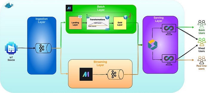
Disclaimer: This is a hypothetical scenario and further development needed to optimize data models, logic and dashboards but I believe it gives a good overview of an end-to-end business case.
Data flow at a glance
Ingestion — Telemetry and event JSON messages are produced by edge devices and land in the Kafka topics
iot‑eventsandiot‑telemetryfor event and telemetry data, respectively.Speed layer — Mage streaming jobs consume
iot‑telemetry, apply real‑time rules, and publish anomalies to a second topiciot‑anomalies. StarRocks ingests that topic into theanomalies_streamingtable and aggregates it in theanomaly_rollupmaterialized view.Batch layer — The same
iot‑telemetryandiot‑eventsstreams are persisted as Parquet in MinIO. Each batch run spins up a Nessie branch, transforms data with Polars, runs QC checks, and materialises three Gold (eg. ready for consumption) tables:gold_device_health,gold_failure_predictions, andgold_maintenance_schedule.Serving layer — StarRocks supports streaming tables, batch tables, and materialized views, providing a single source of truth for dashboards, alerts, and ad‑hoc SQL. Visuals based on Streaming, Batch, and combined sources are shown in Superset
Deeper into the layer
Now, let’s examine how data flows through each layer — from raw ingestion to end-user consumption — and the transformations applied at each stage.
Ingestion layer
This is the part where data is ingested from IoT sensors and simulated using a faked data generator. Below are annotated examples:
Telemetry Data (High-frequency sensor readings)
// Telemetry
{
  "device_id": "device_42",       // Unique machine identifier
  "timestamp": "2025-04-01T09:15:33.456789",  // Precise event time (ISO 8601)
  "energy_usage": 3.78,           // kWh (track efficiency/deterioration)
  "temperature": 24.3,            // °C (critical for overheating alerts)
  "vibration": 1.2,               // mm/s² (high values indicate mechanical stress)
  "signal_strength": 88           // % (monitors connectivity health)
}Purpose: Real-time monitoring of machine health.
Key Alert Triggers: Temperature >28°C, vibration >5 mm/s².
2. Event Data (Batch updates for incidents/actions):
// Failure Event
{
  "device_id": "device_42",
  "event_timestamp": "2025-04-01T09:16:00.000000",  // When failure occurred
  "event_type": "failure",       // Event category
  "severity": "high",            // Impacts alert urgency
  "error_code": "ERR1423",       // Machine-specific failure code
  "component": "bearing",        // Identifies faulty part
  "root_cause": "overheating"    // Helps prevent future failures
}

// Maintenance Event
{
  "device_id": "device_42",
  "event_timestamp": "2025-04-01T10:00:00.000000",  // When maintenance was done
  "event_type": "maintenance",
  "severity": "medium",          // Reflects complexity
  "technician": "tech-15",       // Accountability tracking
  "duration_min": 90,            // Downtime impact analysis
  "parts_replaced": "bearing"    // Inventory/spare parts planning
}Purpose: Logs failures and repairs for trend analysis and compliance.
Pipeline Routing
Telemetry → Kafka topic
iot-telemetry(Speed and Batch Layer for real-time alerts and enrichment of batch data).Events → Kafka topic
iot-events(Batch Layer for historical analytics).
Streaming Layer: Real-Time Anomaly Detection
We process telemetry data in real-time using Mage to detect and alert on critical machine conditions. Here’s how it works:
Stateful Processing:
Tracks the last recorded temperature per device (simple state) to avoid expensive window joins.
Alternative: For complex aggregations, tools like Apache Flink would be needed (beyond Mage’s OSS capabilities).
2. Anomaly Detection Rule (Python Snippet):
if msg.get("temperature", 0) > 28:
            add_anomaly({
                "device_id": device_id,
                "timestamp": msg["timestamp"],
                "anomaly_type": "high_temperature",
                "severity": "CRITICAL" if msg["temperature"] > 32 else "HIGH",
                "description": f"Temperature {msg['temperature']} °C (threshold: 28)",
                "is_confirmed": False,
                "confirmed_by": None,
            })
Why This Matters:
CRITICALalerts (>32°C) trigger immediate shutdown protocols.HIGHalerts (28–32°C) notify maintenance teams for inspection.
3. Output: Anomaly Message
{
  "device_id": "device_42",                  // Machine in distress
  "timestamp": "2025-04-01T10:00:00.000000", // Exact alert time
  "anomaly_type": "high_temperature",        // Standardized for aggregation
  "severity": "High",                        // Prioritizes response urgency
  "description": "Temperature 32 °C (threshold: 28)", // Context for ops teams
  "is_confirmed": False,                     // Flagged until reviewed
  "confirmed_by": None                       // Audit trail post-review
}Destination: Published to Kafka topic
iot-anomalies→ StarRocks for live dashboards and alerts.
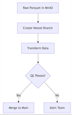
Batch Layer: Versioned Data Pipelines
We transform raw IoT data into three business-critical tables using Polars + PyIceberg, with Nessie providing Git-like version control. Here’s the complete workflow (For more details about setting up Nessie you can refer to this post):
For simplicity, we skip a full medallion (Bronze/Silver/Gold) architecture. The Write‑Audit‑Publish (WAP) pattern via Nessie already gives atomicity and rollback safety.
Gold Tables Implementation
We have three Gold tables that we will use for the final dashboard.
gold_device_health(Machine Health Snapshot):
device_id(string): Unique machine IDdate(date): Partition dayavg_energy(double): Mean kWh/daymax_temp(double): Highest °C/daymin_health_score(double): 0–1 diagnostic score (lower = worse)vibration_anomalies(int): Count of vibration spikestemp_anomalies(int): Count of temperature spikesdays_since_maintenance(int): Rolling counter since last maintenancefailed_components(array): Components that failed that day
@transformer
def transform(silver_telemetry, silver_events, *args, **kwargs):

    telemetry_daily = silver_telemetry.group_by(["device_id", "date"]).agg([
        pl.col("energy_usage").mean().round(2).alias("avg_energy"),
        pl.col("temperature").max().alias("max_temp"),
        pl.col("composite_health_score").min().alias("min_health_score"),
        pl.col("is_vibration_anomaly").sum().alias("vibration_anomalies"),
        pl.col("is_temp_anomaly").sum().alias("temp_anomalies"),
        pl.col("signal_strength").mean().alias("avg_signal_strength")
    ])

    ##### FULL CODE CAN BE FOUND IN THE REPOSITORY#######
    # Fill nulls separately for each column
    return result.with_columns([
        pl.col("failures_count").fill_null(0),
        pl.col("failed_components").fill_null([]),
        pl.col("days_since_maintenance").fill_null(999)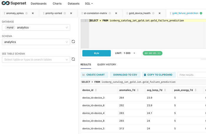
])gold_failure_predictions(Risk Scoring):
device_id(string)prediction_date(date): Forecast horizonfailure_risk_score(double): Probability 0–1anomalies_24h(int): Recent anomalies in the last 24 hpeak_temp_24h(double): Highest temperature in the last 24 hrecommended_action(string): e.g. “replace bearing”
@transformer
def transform(device_health, silver_telemetry, *args, **kwargs):

    current_date = datetime.now().date()
    lookback_7d = silver_telemetry.filter(
    pl.col("date") >= (current_date - timedelta(days=60))
    ).group_by("device_id").agg([
        pl.col("is_vibration_anomaly").sum().alias("anomalies_7d"),
        pl.col("temperature").mean().round(1).alias("avg_temp_7d"),
        pl.col("energy_usage").max().alias("peak_energy_7d"),
        pl.col("composite_health_score").min().alias("worst_health_score_7d")
    ])

    ##### FULL CODE CAN BE FOUND IN THE REPOSITORY ####

    # Then add the recommended_action based on the failure_risk_score
    data = data.with_columns(
        pl.when(pl.col("failure_risk_score") > 0.8).then("immediate_shutdown")
        .when(pl.col("failure_risk_score") > 0.6).then("emergency_maintenance")
        .when(pl.col("failure_risk_score") > 0.4).then("schedule_maintenance")
        .otherwise("monitor_only")
        .alias("recommended_action")
    )
    print(data.columns)
return datagold_maintenance_schedule(Repair Planner):
device_id(string)priority(string): P0 (immediate) … P3window(string): e.g.within_4_hoursestimated_cost(int): USDfailure_risk_score(double): Copied from predictions
@transformer
def transform(failure_predictions,device_health, *args, **kwargs):

    # First create the priority column
    data = device_health.join(failure_predictions, on="device_id", how="inner")
    data = data.with_columns(
        pl.when(pl.col("failure_risk_score") > 0.7).then("P0")
        .when(pl.col("days_since_maintenance") > 90).then("P1")
        .when(pl.col("vibration_anomalies") > 5).then("P2")
        .otherwise("P3")
        .alias("priority")
    )

    ###### FULL CODE CAN BE FOUND IN THE REPO #####

    # If you want to expand the struct, do it after selecting
    data = data.with_columns(
        pl.col("suggested_intervention").struct.rename_fields(["window", "estimated_cost"])
    ).unnest("suggested_intervention")

    return data
Serving Layer
The serving layer is where final outputs — batch-processed, streaming, and unified data — are exposed for consumption. This is the point where processed data becomes available through queries and visualizations.
In this implementation, we use StarRocks to power a high-performance analytics engine and Apache Superset as the front-end visualization tool.
🟢 Streaming Data
We start by ingesting anomaly data in near real-time using StarRocks’ ROUTINE LOAD from Kafka.
1. Create the target table
-- Table creation
CREATE TABLE anomalies_streaming (
    device_id STRING,
    timestamp DATETIME,
    anomaly_type STRING,
    severity STRING,
    description STRING,
    is_confirmed BOOLEAN,
    confirmed_by STRING NULL

    )
PRIMARY KEY (device_id, timestamp)
PARTITION BY date_trunc('day', timestamp)
DISTRIBUTED BY HASH(device_id)
ORDER BY (timestamp, severity)
PROPERTIES (
    "enable_persistent_index" = "true",
    "replication_num" = "1"
);
2. Load from Kafka
-- ROUTINE LOAD TO INSERT DATA FROM KAFKA TO STARROCKS
CREATE ROUTINE LOAD iot_anomalies_load ON anomalies_streaming
COLUMNS (device_id, timestamp, anomaly_type, severity, description, is_confirmed, confirmed_by)
PROPERTIES (
    "desired_concurrent_number" = "1",
    "format" = "json",
    "jsonpaths" = "[\"$[*].device_id\", \"$[*].timestamp\", \"$[*].anomaly_type\", \"$[*].severity\", \"$[*].description\", \"$[*].is_confirmed\", \"$[*].confirmed_by\"]"
)
FROM KAFKA (
    "kafka_broker_list" = "kafka:9093",
    "kafka_topic" = "iot-anomalies",
    "property.kafka_default_offsets" = "OFFSET_END"
);
3. Managing the stream
Once you execute the ROUTINE LOAD above, you can use the following commands to debug, restart, or stop the load.
-- Helpful commands to debug routine load
SHOW ROUTINE LOAD FOR iot_anomalies_load

STOP ROUTINE LOAD FOR iot_anomalies_load

RESUME ROUTINE LOAD FOR iot_anomalies_load
To simplify UI queries and reduce dashboard latency, we define a materialized view (materialised views can be Synchronous or asynchronous) that aggregates anomalies over hourly buckets:
CREATE MATERIALIZED VIEW anomaly_rollup
DISTRIBUTED BY HASH(device_id)
REFRESH ASYNC EVERY (INTERVAL 15 MINUTE)
AS
SELECT
    device_id,
    DATE_TRUNC('hour', timestamp) AS hour_bucket,
    COUNT(*) AS total_anomalies,
    COUNT_IF(is_confirmed = false) AS unconfirmed_count,
    COUNT_IF(severity = 'high') AS high_severity_count,
    ARRAY_AGG(DISTINCT anomaly_type) AS anomaly_types
FROM
    anomalies_streaming
GROUP BY
    1, 2;
This view is refreshed asynchronously every 15 minutes to balance freshness and performance.
📦 Accessing Batch Data
Our batch-processed tables (e.g., gold_device_health) are stored in Iceberg format on MinIO. These cannot be queried directly through Superset if you're connected via StarRocks.
Instead, you can:
Run SQL queries in Superset using StarRocks’ Iceberg integration (after linking the external catalog -> check post here.).
Optionally, define synchronous materialized views in StarRocks that mirror batch tables for direct use in dashboards (I haven’t experimented with that option yet).
🔀 Combining Batch and Streaming
Merging batch and streaming views in a unified query is often a challenge with table formats. Fortunately, StarRocks allows us to build a consolidated materialized view that joins both:
-- Hourly refreshed view combining batch and streaming
CREATE MATERIALIZED VIEW unified_device_health
REFRESH ASYNC EVERY (INTERVAL 1 HOUR)
AS
SELECT
    b.device_id,
    b.date,
    b.min_health_score AS health_score,
    b.days_since_maintenance,

    -- Streaming metrics directly from anomalies_streaming
    COUNT_IF(s.is_confirmed = FALSE) AS pending_anomalies,
    COUNT_IF(s.is_confirmed = FALSE AND s.severity = 'high') AS urgent_anomalies,

    -- Criticality Score
    ROUND(
        ((1 - b.min_health_score) * 0.6) +
        (LEAST(COUNT_IF(s.is_confirmed = FALSE), 10)/10.0 * 0.3) +
        (CASE WHEN b.days_since_maintenance > 90 THEN 0.1 ELSE 0 END),
    2) AS criticality_score,

    -- Priority logic
    CASE
        WHEN (1 - b.min_health_score) > 0.7 OR b.days_since_maintenance > 120 THEN 'P0'
        WHEN (1 - b.min_health_score) > 0.5 OR b.days_since_maintenance > 90 THEN 'P1'
        WHEN b.vibration_anomalies > 5 OR b.temp_anomalies > 3 THEN 'P2'
        ELSE 'P3'
    END AS priority

FROM
    iceberg_catalog_iot_gold.iot.gold_device_health b
LEFT JOIN
    anomalies_streaming s
    ON b.device_id = s.device_id
    AND DATE_TRUNC('day', s.timestamp) = b.date

GROUP BY
    b.device_id,
    b.date,
    b.min_health_score,
    b.days_since_maintenance,
    b.vibration_anomalies,
    b.temp_anomalies;
This view enables daily-refresh dashboards that merge long-term health metrics with recent alerts to guide maintenance decisions.
Materialized views can accessed directly from Superset as they are stored in StarRocks.
📊 Dashboards in Superset
The final step on the serving layer is some sort of dashboard that end users can use to get some information about the devices in the manufacturing plant.
To display any data, you will need to establish a connection first as follows:
In Superset, go to Settings → Database Connections.
Choose “Other” as your database type.
Set your SQLAlchemy URI (e.g.):
mysql+pymysql://root:@starrocks-fe-0:9030/analytics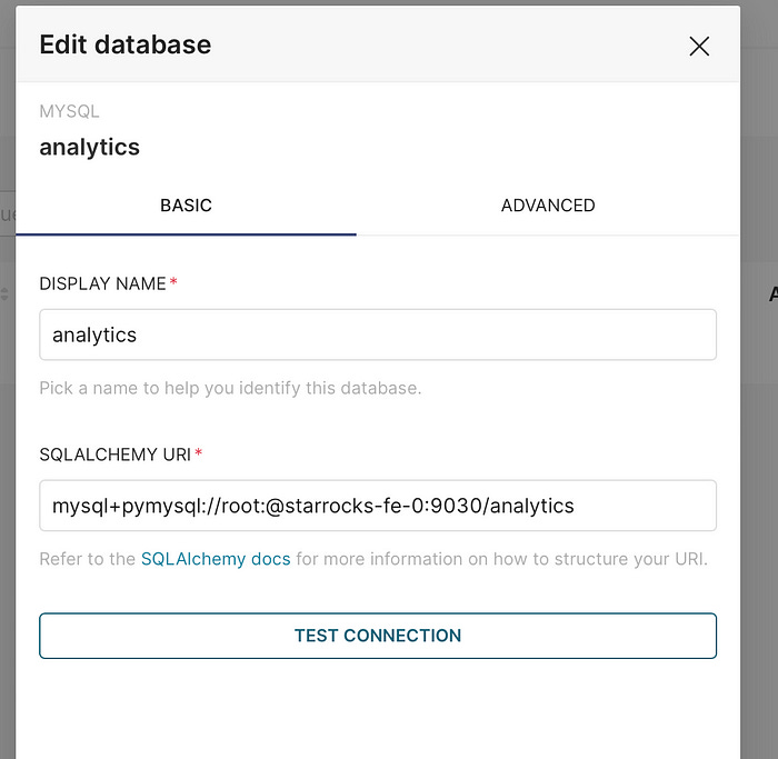
Once connected, you can explore tables like unified_device_health and anomaly_rollup to build dashboards.
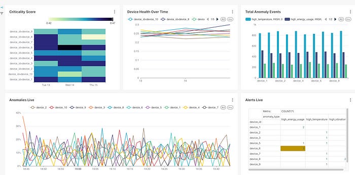
Of course, having a longer time span of data would improve the quality and depth of insights. The more data we collect, the more meaningful our analysis becomes. That said, even with limited data, we can already observe useful patterns. For example, on the 14th of the month, device_6 was in a highly critical state. Then, on the 15th at around 19:50 (as shown in the bottom-right live alerts panel), the same device triggered three high_temperature alarms—an event that should prompt immediate attention from the operations team.
Conclusion
Throughout this tutorial, I aimed to walk you through all the key components required to build an end-to-end data pipeline using the Lambda Architecture.
We explored how to use Polars for efficient data transformations, PyIceberg for managing Iceberg tables, and the Nessie catalog for versioning and ensuring data accuracy through the Write-Audit-Publish (WAP) pattern. While the streaming layer is intentionally kept simple, it demonstrates the core building blocks for real-time processing — though for more advanced needs, tools like Apache Flink may be more appropriate.
We also covered how to use materialized views in StarRocks to speed up both visualizations and SQL queries. If you’re looking for more real-world examples of this, check out reference [4].
Finally, while the IoT scenario used here is hypothetical (and may luck some business details), it’s a practical way to tie the architecture together. In reality, gathering and refining business requirements is often one of the hardest parts of any project.
I hope you found this post insightful!
Feel free to connect with me on LinkedIn, and don’t forget to check out the GitHub repository for the full code and other data engineering projects.